Math for Machine Learning: Series 3 — Probability & Statistics

From Bayes’ Theorem to Maximum Likelihood — The Mathematics of Uncertainty

Jul 07, 2026

If you missed them, here are the first two parts of the curriculum:

Series 1: Linear Algebra (How data is structured and transformed)
Series 2: Calculus of Deep Learning (How models learn and optimize)

Series 3 completes the trilogy.

In programming, logic is deterministic. if x > 5 is always true or always false. But machine learning operates in the real world; a world of noise, missing data, and educated guesses. To build models that work in the real world, we have to stop thinking in certainties and start thinking in bets.

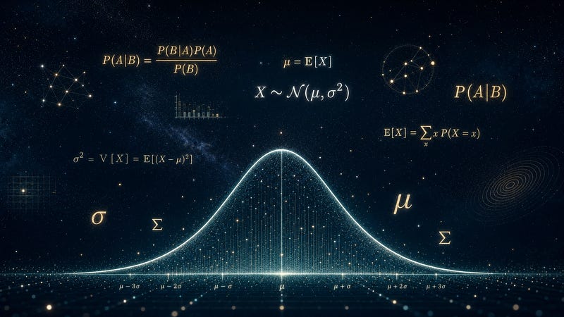
This series covers the probability and statistics that form the foundation of statistical learning.

Why This Series Exists

Why do we use Mean Squared Error for regression? Why do we use Cross-Entropy for classification? Why do we add an L2 penalty for regularization?

If you treat machine learning as a black box, these are just arbitrary formulas you memorize. But they are not arbitrary. They are mathematically derived from probability theory.

When you understand the statistics behind the loss functions, you stop guessing which one to use. You know exactly what assumptions your model is making about the world, and you know how to fix it when those assumptions are wrong.

The Learning Path

Article 1: Thinking in Bets

Bayes’ Theorem from Scratch

We start by shifting from deterministic to probabilistic thinking. We tackle the counterintuitive nature of probability using the famous medical test paradox.

You will learn:

Why a 95% accurate test can mean you are probably fine. The Prior, the Likelihood, and the Posterior. How Bayes’ Theorem is just a formal way of counting areas. How to build a Naive Bayes spam filter from scratch in NumPy.

Key insight: Bayes’ Theorem is the mathematical engine for updating your beliefs when you see new evidence.

Article 2: The Shape of Chaos

Why the Normal Distribution Rules Machine Learning

We move from discrete counting to continuous measurements. We explore why one specific shape, the bell curve, dominates the physical universe and machine learning.

You will learn:

The difference between discrete probabilities and continuous densities. The parameters of the Gaussian distribution. The Central Limit Theorem, simulated with dice rolls. Why the errors in your data are almost always normally distributed.

Key insight: The Normal distribution is not an arbitrary choice; it is the mathematical shape of chaos averaging out.

Article 3: The Search for Truth

Maximum Likelihood and MAP Estimation

We put it all together to answer the ultimate question: what does it actually mean to “fit” a model to data?

You will learn:

How to find the parameters that maximize the probability of your data (MLE). Why minimizing Mean Squared Error is mathematically identical to MLE under Gaussian noise. The flaw of MLE (no common sense). How Maximum A Posteriori (MAP) estimation fixes this by adding a Prior. Why L2 Regularization is mathematically identical to a Gaussian prior.

Key insight: You are not just drawing a line of best fit. You are finding the parameters that make your observed data the most statistically probable outcome in the universe.

The Complete Picture

By the end of Series 3, you will see how the three pillars of machine learning math connect.

You use Linear Algebra to structure your data. You use Probability to define your loss function (MLE/MAP). You use Calculus to minimize that loss function.

They are not separate subjects. They are a single, coherent framework.